Validation of calculation algorithm for clinical IMRT cases
Test purpose
Validation of calculation algorithm for wide spectrum of clinical cases, including plans with long (>26 cm) field sizes.
Test method
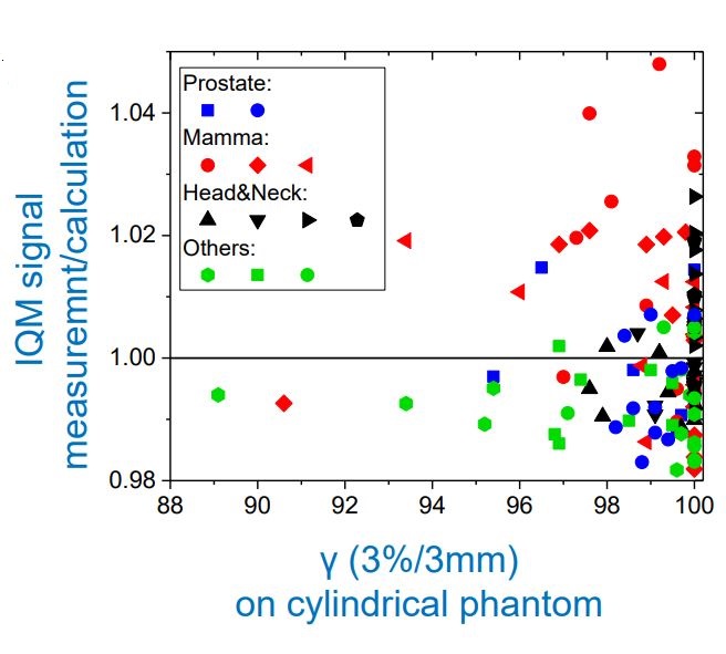
More than 100 fields of different plan types were measured and compared against the results calculated by the IQM calculation algorithm.
Test results
The overall agreements of the measured signal with the calculated signal was -0.2% (±1.3%). For long (> 26 cm) field sizes the agreement of the measured signal and the calculated signal is +0.4% (±1.4%).
Conclusion
IQM signal measurements agree well with the calculated references. The difference between the measured and the calculated reference signal for long field IMRT beams was slightly larger than for smaller IMRT fields. IQM can be used to verify field size of up to 40 cm x 40 cm. Very limited user interaction was necessary to achieve these results.
The physics behind the IQM Signal
Scope
Outline the calculation model for IQM in terms of the physical characteristics and behavior of linear accelerators.
Expected inputs for signal prediction
- Chamber characterization
- Treatment unit (Linac) characterization
- Collimation attenuation
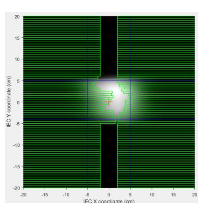
- Fluence profiles
- Patient treatment description
- Both static field-in-field and dynamic delivery modes
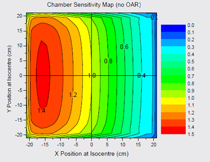
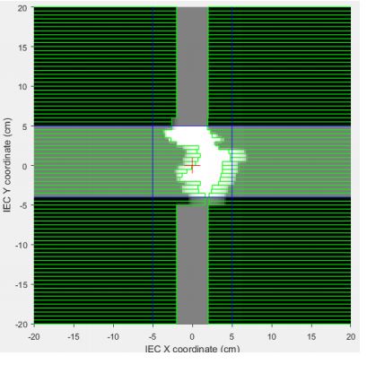
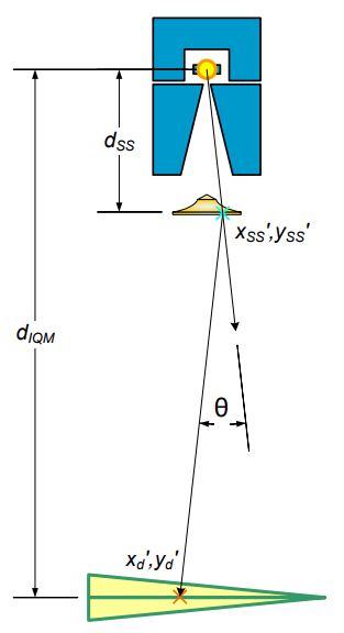
IQM chamber properties
- Sloped electrode chamber
- Spatial gradient = delivery position encoding
- Characterized by
- Reference field normalization
- Gradient (sensitivity) map
- CSM, (????)
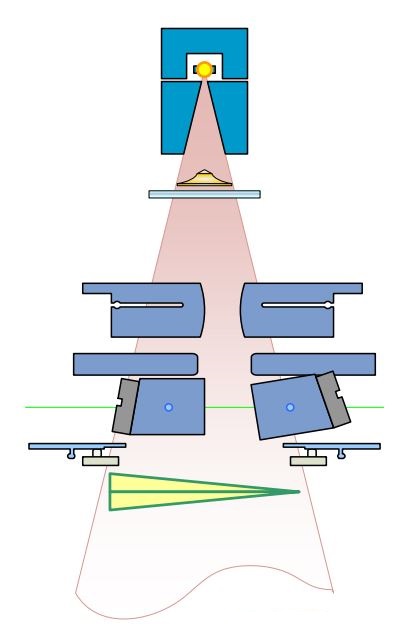
Linac characterization
- Behaviour to capture
- Output change with field size
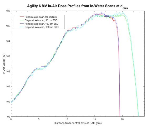
- Radial Profile
- Transmission through collimating elements
- Source Assumption
- Primary point source
- Extended secondary source
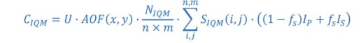
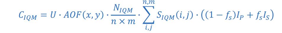
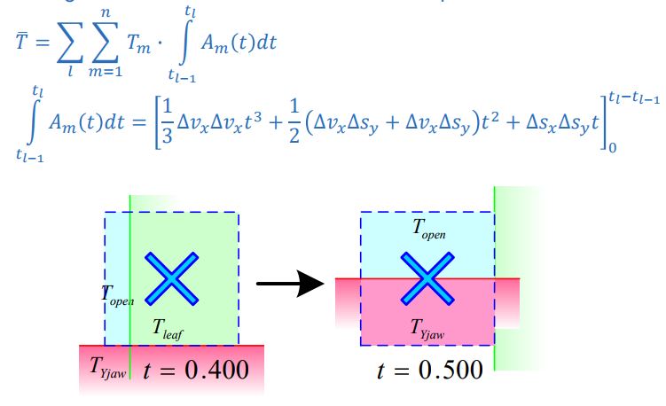
Fundamentals of signal calculation
- ? = MU setting for segment
- ??? = output change with field size (residual…)
- ???? / ?×?= normalization (electrometer reading)
- ?p, ?s = primary and secondary source intensity matrix
- ?? = fractional contribution from secondary source
- ???? = chamber positional sensitivity matrix
Primary source intensity
- Starts with open source profile
- Assume radially symmetric intensity profile
- Apply effect of collimation attenuation
- Works on an area weighted average rather than an intensity to a point
Primary Source Modulation
- Area-Weighted Transmission through collimating elements subdivided in regions of transmission and time for each pixel
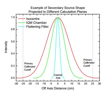
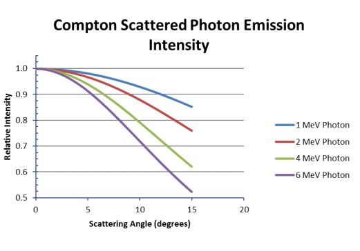
Secondary source
- Extended source geometry
- Positioned at bottom of flattening filter
Secondary source modulation
- More complex geometry
- Non-divergence matched
- Multiple off-axis sources
- Complex element shape shading
- Simplify calculation
- Static “snapshot” calculation
- Sampling point geometry
- Layered collimating element
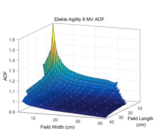
Area output factor characterization
- Captures changes in output due to field size effects
- Derived from a series of rectangular field measurements
- Behaves as a “residual”
- Some effects accounted for byextended source
- Rederived for tweaks in source description & transmission
- Look-up according to average field width, length